size of Canada

9.98M km²

Geodesy

The study of the Earth's shape, orientation in space, and variations in gravity

The Earth is not a perfect sphere

Ellipsoid (Spheroid)

A model of the Earth that uses sea level as a base

Geoid

Datum

A mathematical reference surface, or model, used for plotting locations. Can be either global or local in coverage.

Datums are based on these

a region of best fit

region of best fit

an imaginary ellipsoid that best regionally fits the Geoid.

Datum transformation

A series of calculations that convert datums from one to another

Two Datum transformation systems developed by Canada and the US

WGS84 and NAD83

The earth Bulges at the... because...

equator due to rotational forces

Datums are used to...

establish Geographic Coordinate systems (GCS)

Geographic coordinate system (GCS)

A global reference system used for determining locations on an ellipsoid

Longitude

imaginary lines on a globe running from pole to pole describing location from East to West

The prime meridian is numerically known as this

the origin, or zero degrees

Latitude

Imaginary lines on a globe running from East to West describing location from North to South

The equator is numerically known as this

The line of Origin or zero degrees

the equation(s) for converting DMS into DD

D + (M/60) + (S/3600) or D + ((M+S)/60)/60

Another word for an ellipsoid

Spheroid

- 42.15188^o

42^o 9' 6.788" W

130.6790^o

130^o 40' 44.4" N

Projection

A mathematical process of converting a 3d model of Earth into a 2d map of Earth

three basic kinds of developable surfaces for casting projections

Azimuthal, Conical, and Cylindrical

the three commonly used development surface orientations

Normal, Transverse, and oblique

Downside of Lambert Conformal Conical Projections

LCCPs are not suitable for larger areas because it only minimizes distortion locally.

What projection type is a Lambert conformal?

Conical

A great use for Mercator Maps

MMs are good for things like navigating by compass because it minimizes straight line distortion.

A trade off of using a Mercator Projection

They sacrifice accuracy of depictions of area on a map to project straight lines more accurately.

Peter's Projection

A projection that most accurately depicts area on a map while maintaining minimum distortion

Projected Coordinate System (PCS)

A coordinate on a flat 2d surface. The Surface has constant lengths, angles, and areas.

Universal transverse Mercator (UTM)

an international coordinate metric system

60 UTM zones consisting of this many degrees each

6 degrees of longitude per zone

areas not included in UTM

above 84 degrees N and 80 degree S of latitude

UTM meridians count starting at this meridian

East from the 180th Meridian

UTM zone coordinates are measured in this unit

Meters

Northings

Distance N or S of the equator

Eastings

the distance E or W from the central meridian or the False Easting

Each UTM zone has a central meridian with this value

500,000m

UTM locations on this side of a zone's central meridian are subtracted

Locations west of the central meridian

The names or codes for a UTM Location always contain this

Zone Number

Dominion Land Survey (DLS)

A system developed by Canada that makes UTM zones line up for easier usage.

The seven meridians of the DLS from East to West

West of Winnipeg, Manitoba/Sask Border, Moose Jaw Sask, Sask Alberta Border, Calgary (Barlow Trail), and Grand Prairie

The Base unit of Measure in DLS

Township (6 x 6 miles)

there are two of them to the N and S of each baseline in DLS

tiers of township

East and West edges of a township

Defined as lines of longitude

used to designate townships

Township numbers and range numbers

Township numbers

They start just North of the first baseline and increase going North

Recommence at every meridian and increase going west

Range numbers

Meridians are not referenced in this province

Manitoba

equal to a township

36 sections

equal to a section

4 quarter sections or 16 Legal Subdivisions (LSDs)

Global Positioning System (GPS)

Technology that broadcasts satellite signals for navigation and position determination on Earth

Transit or NAVSAT (1964)

tracking for military and commercial sea vessels

NAVSTAR (1973)

a GPS system developed by the US that implemented a navigating system that had timing and ranging.

1978

the first four satellites were launched

1983 (two things happened)

The soviet union shoots down North Korean air lines flight 007 after it flew off course.

The US makes it's GPS system globally available.

1990

first usages of selective accessability

1993

the 24th satellite is launched and is fully operational by 1995

2000

Differential GPS services make selective accessibility less effective

Global navigation satellite systems (GNSS)

Overall term for technology that uses satellite signals to find locations on Earth.

Three segments of GPS

Space, Control, User

amount of satellites needed for an effective GPS satellite constellation

24 Satellites

Orientation of a GPS Satellite constellation

orbit altitude of 20,200km, six orbital planes separated by 60 degrees

Ephemeris

Information about the satellite's status, orbit, and precise location information

The Ephemeris of a signal contains two pieces of information

Signal containing Satellite position and its precise time of transmission

Each satellite has a unique signal

Pseudo-Random code

C/A Code (Coarse acquisition)

L1 frequency information that is available for all GPS users

L1 frequency

Navigation information (time and position)

P-Code (precise)

L1 and L2 frequency information available to military recievers

L2 frequency

Measures atmospheric interference

Y-Code

encrypted version of P-code intended for military use

User segment

GPS receivers on the ground that pick up satellite signals

The number of Satellites is controlled by this

The number of Channels

A twelve channel receiver can pick up signals from this many satellites

12 Satellites

Single Frequency Receiver

Receivers that only use the L1 frequency

Dual Frequency Reciever

Receivers that use both L1 and L2 frequencies

Trilateration

A process of finding a position based on its distance from three or more other known points

3D Trilateration

term for finding a point on the Earth's Ellipsoid surface using Trilateration

Pseudo Range

The distance between a GPS receiver and satellite

Equation for Calculating Pseudo Range

PR= c x Transmission time

used to correct time errors and find a vertical location

A fourth GPS Satellite

Clocks used by Satellites

Atomic Clocks

Clocks used by Receivers

Quartz Clocks

Five Sources of error in GPS'

TDOP, PDOP, atmospheric interference, multipath signals, and selective availability

Five factors that influence Position Dilution of Precision (PDOP)

• Error introduced due to the geometric position of satellites
• A wide distribution of satellites results in higher position accuracy
• GPS receivers can select satellites based on position
• Some receivers will calculate the range of PDOP
• Other receivers may allow users to select satellites

GPS Satellites that are closer

have Poor Geometry, are less accurate

GPS Satellites that are farther apart

have Good Geometry, are More accurate

Ionospheric errors

Refraction and slowing of GPS signals can cause roughly a 5m error in pseudo range

Tropospheric errors

refractions can cause up to 0.5m errors in pseudo range

Multipath Signals

Error caused by the reflection of GPS signals from surrounding surfaces. effect can be combatted by raising the height of the receiver antenna or dish.

Selective availability

Sometimes intentional degradation of the timing and location of GPS satellite information which can limit C/A code accuracy to about 100m

Differential GPS (DGPS)

A method of using ground-based corrections in addition to satellite signals. They work best when they are closer to receivers. reduces error to ~5m

Real time kinematic (RTK)

Combination of GPS signals and a base station to provide real-time corrections. Commonly used for mobile data connections

Post processed kinematic (PPK)

Combination of GPS signals and a base station to correct location information after data collection

Wide area augmentation system (WAAS)

A network of ground stations that measure variation in GPS signal. reduces error to ~3m

Three principles of map design

Generalization, Simplification, and Symbology

Map

represents spatial data that provides a reader with information. They can be abstract representations of the real world. A complex model of reality.

Cartographic generalizations

The simplification of representing items on a map. often controlled by a scale

Douglas-Peucker Simplification (line simplification)

curved lines are simplified based on a set of defined points

Displacement

describes how features can be moved slightly to increase clarity. (smoothing or enhancement)

tree methods of generalization

Line simplification, reduction of spatial complexity, symbology

Geographic scale

The real-world size or area of a feature. Larger objects on the ground have a larger geographic scale.

Map Scale

A value representing the number of units on a map relative to the number of the same units on the ground

Representative Fraction

The number of units on a map Vs. the number of the same units on the ground. These are unitless values.

Verbal Scale

Using relatable units on both sides of the relation

Scale bar

A graphic representation of the map scale

Large scale Maps

Maps showing a small geographic region with a large RF value.

Small scale Maps

Maps showing a large geographic region with a small RF value

Accuracy

The degree to which information in a map or a digital database matches true values (refers to data quality and the number of errors in a dataset)

Precision

The level of measurement exactness or repeatability of a dataset. (no. of significant digits used.)

The half millimeter rule

The area of uncertainty increases as scale increases.

Reference Map

A map that shows where geographic features are in relation to each other

Thematic Map

A map designed to convey information about a single topic

Topographic Maps

These maps have strict rules about how they are made

Symbology

The set of conventions or rules that define how geographic features are
represented with symbols on a map

Single symbol

Symbology method where all features draw in the same color and symbol

Unique values

Symbology method where features draw differently based on category or type attribute

Graduated Colours

Symbology Method where features are placed in classes based on numeric values

Graduated symbols

Symbology method where features are placed in classes based on numeric values and symbol size reflects class value

Classification (Symbology)

Features are divided by numeric values into classes. Has a large range of classifying methods. Only used together with Graduated Symbology.

Natural breaks

Determines classes based on the natural grouping of the data

Jenks

Another name for natural breaks

Quantile

Each class contains an equal number of features

Equal interval

Divides the range of values into equally sized subranges

pros/cons of Natural breaks

• Good for mapping uneven distributions

• Not good for comparing data

• Difficult to determine the proper number of classes

pros/cons of Quantile

• Provides an understanding of relative position

• Similar features may end up in different classes

• Wide range of values may end up in the same class

pros/cons of Equal interval

• Best for familiar values such as percentages or temperature

• Prone to issues with clustering

• Not ideal for uneven distributions

Normalization

• Doing this to data creates a ratio map
• Allows for comparison between different areas

Nine components of a map for this class

1. Title
2. Data frame
3. Scale
4. Legend
5. Descriptive text
6. North arrow
7. Sources
8. Name, date, class number
9. Neatline

Six essential components for a map

1. Title
2. Data frame
3. Scale
4. Legend
5. Descriptive text
6. North arrow

Data frame

• Data portion of a map
• Consider the purpose of your map when selecting what and how much you show

Do not abbreviate this

A legend on a map

What research Dr. John Snow did during the 1854 cholera outbreak in London

Mapped the locations of outbreaks in London and examined the relationship between outbreak locations and things like road networks, neighborhoods, and water sources.

Miasma theory

• “Night air” or “Bad air”
• Belief that disease was called by smell
• Cesspools were emptied into the river
• Cholera outbreaks increased

Germ theory

• Microorganisms can affect diseases
• Proposed in the 1500s, accepted in the 1880s

This was patient zero according to Dr. Snow

Baby Lewis

Dr. Snow's Solution to the London outbreaks of 1854

The outbreak was centered around the Broad Street water pump. Dr. Snow convinced the Parish Board of Governors to remove the pump handle.

Dr. Snow is considered the first in this field of battling disease outbreaks

The first epidemiologist

The Grandfather of GIS

Ian McHarg

Some things Ian McHarg did

• Author on landscape architecture and regional planning
using natural systems.
• Pioneered the concept of ecological planning with his
book Design with Nature (1969).
• Argued that humans should integrate with nature and
strongly opposed the idea of subjugating nature.
• Fundamental in forming the basic concepts used in
geographic information systems.

Sieve Mapping

Analysis of an area based on layers made up of certain features that can be removed or added to show their relationships

The Father of GIS

Roger Tomlinson

Some things Roger Tomlinson did

• Created the Canadian Geographic System (CGIS) in 1962
• The first operational GIS
• CGIS used a layered approach to mapping
• Used to store geospatial data for the Canada Land Inventory

Howard Fisher

Created SYMAP; one of the first computer mapping software's in 1964

GIS focused institution established in 1965

Harvard Laboratory for Computer Graphics

In 1969, Jack and Laura Dangermond founded this institute

Environmental Systems Research Institute (ESRI)

ESRI (Environmental Systems Research Institute)

An institution that applies mapping and spatial analysis to help land resource managers make decisions.

ARC/INFO

The first commercial GIS product first released in 1981

Crowd Sourcing

• Geolocation data collected from portable technology
• Contributions to OpenSteeetMap, geotagged images, business tracking

The Geospatial Cloud

•Increased operational efficiency
• Development of two-way data communication
•Analyze large datasets

GIS Software

• Computer-based hardware and software used to capture, analyze, manipulate, and visualize geospatial data.
• The ability to handle spatial data separates GIS from other software.

Three words to summarize the advantages to using GIS software

Toolbox, Database, Organization

Geographic Data

• Any data with spatial coordinates
• Points, lines, polygons, rasters

Information Data

• Databases and data integration
• Non-spatial data (e.g., Income data, average revenue, population, age…)

System Data

• Integration of data and tools
• Hardware, software, toolboxes, printers, and users

Five steps to the geographic approach

1. Ask
2. Acquire
3. Examine
4. Analyze
5. Act

GIS software's can be broken down into 7 main features

• data collection
• storage and management
• Data retrieval
• Data conversion
• Analysis
• Modeling
• Display

Metadata

Descriptive information about a data file

Metadata can include:

• Identification numbers
• Data quality and accuracy
• Spatial organization (vector or raster)
• Spatial reference data
• Description of each attribute
• Where data can be found
• Citations
• Contact information

Geodatabase

Single folder that can hold numerous files with almost unlimited space

Feature Class (geodatabase)

Single data layer (point, line, or polygon). Also stores raster, CAD files, tables, etc

Feature dataset (geodatabase)

Grouping of multiple feature classes. Effective way of storing and sharing data

This is an image of a Geodatabase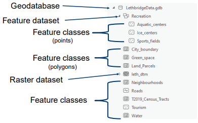

Catalog

allows you to view, create, and manage items in your project

7 file types and their uses

• .cpg – Characters used to display text
• .dbf – Stores attributes
• .prj – Stores coordinate system information
• .shp – The main shapefile
• .shx – The index of the feature geometry
• .ovr – The compression and quality of
rasters
• .rrd – reduced-resolution of rasters

Layer Package

• Shares just one layer
• Includes properties and data for a layer

Map Package

• Shares an entire map
• Includes properties and data for layers in a map

Project Package

• Share the entire project
• Includes properties and data for layers in all maps
• Stores toolboxes, databases, styles, models, and more

Web Layer

• Shares data layers in a map as web layers

Web Map

• Shares an entire map and creates a web map

Discrete View (Discrete object view)

Representing the world with a series of separate objects.

• Points: A simple set of coordinates
• Lines: A one-dimensional object that connects starting and endpoints
• Polygons: A two-dimensional object that forms an area from a set of lines

Continuous View (Continuous field view)

Viewing the world as items that vary across the Earth’s surface as constant fields

Continuous view (Raster data model)

Spatial model that uses an array of equally sized cells arranged in rows and columns

Naming Restrictions for a raster data model

• Maximum of 13 characters
• Cannot start with a number
• No spaces
• Underscore is the only character that can be used
• File path cannot be more than 128 characters

pro's of Vector data

• No generalization
• Aesthetically pleasing
• Accurate geographic locations
• Can store many attributes

Con's of Vector data

• The location of each vertex is stored explicitly
• Not effective for continuous data
• Spatial analysis within a polygon is not possible

Pro's of Raster data

• The location of each cell is implied by its location in the grid
• One attribute per cell is ideal for mathematical modelling
• Represent continuous data

Con's of Raster data

• Cell size can result in block images
• Poorly represents linear features
• Files can be large
• Spatial inaccuracies

Attribute

Non-spatial data associated with a spatial location. Attributes are stored in an attribute table.

The amount of attributes a piece of vector data can have attached to one location

Many can be assigned (Numerous)

Joins

a method of linking two (or more) attribute tables
•Attribute tables must share a common field
•Your “join table” will be added to your “input table” based on the common field
• Joins may be removed once created

Relates

• Defines a relationship between two or more tables but does not attach or move data
• Requires a common field
• Can be a preferred method if working with one-to-many relationships or numerous tables
• Relates can be undone

Spatial Join

Used when layers do not have a common attribute field

Spatial Join (one-to-one)

A Join Operation that summarizes the joining information with each feature in the target layer

Spatial Join (one-to-many)

A Join Operation where If multiple join features overlay the target feature, the output will contain multiple copies of the target feature.

Selections

•Interactive selection
• Used on a map or attribute table
• Database query “Select By Attributes”
•Spatial query “Select By Location”
• Use the clear button to remove selections

Database Query

Computer language with defined syntax used for accessing data from databases

Language used by Database Query's

Structured Query Language (SQL)

Format of an SQL statement

<Field_Name><Operator><Value or String>

• Text variables must be in ‘ ‘
• Enter the Boolean operator if multiple criteria are required

Compound Query

A query used to make selections based on multiple criteria.

selects the intersection between multiple criteria

AND

selects everything that meets both criteria. Can be referred to as a union

OR

selects what meets the first criteria but not the second criteria. This can be referred to as negation

NOT

selects all features that only meet the first and second criteria. This can be referred to as exclusive

XOR

Spatial Query

Selecting features or information based on a spatial relationship

Intersect

Selects features in the input layer that completely or partially overlap the selecting features

Within a Distance

• Creates a search area from the selecting feature
•Selects input features that fall within that search area
•Example: Select buildings within 1000 m of a railroad

Within

Selects input features that are located completely or partially within the selecting
feature.

Completely Within

•Selects the input feature if it does not share a boundary with the selecting feature.
•Alberta is within Canada
•Alberta is not completely within Canada

Contains

•Selects the input feature that has the selecting feature within it.
•Inverse of within
• The United States contains Texas

Completely Contains

• The selecting feature must be completely within the input feature
•Input must be a polygon
•Inverse of completely within
• The United States contains Texas
• The United States completely contains Kansas

Boundary Touches

•Selects the input if it touches the boundary of the selecting feature
•Input and selecting features must be lines or polygons
• The United States, Guatemala, and Belize touch the boundary of Mexico

Copy Feature

• Copies but does not save the new shapefile
• Right-click on the layer → Selection → Make a layer from selected features
• Copy features tool (Data Management Tools)

Export Feature

• Converts a shapefile to a new shapefile based on the selection
• Allows you to output the data
• Right-click on the layer → Data → Export data

Digitizing

Process of creating points, lines, or polygons which represent features from a map or image. Errors can propagate during digitizing

needed for Heads down Digitizing

Obsolete method of digitizing

• Digitizing tablet
• Hardcopy map

needed for Heads up Digitizing

Newer method of digitizing

•On-screen
•Satellite images, air photos, or scanned maps

Heads down Digitizing

• Named based on the position of the user's head while digitizing
• Tablets use a grid of wires to generate a magnetic field which is detected by the cursor.
• Tablet accuracies are about 0.1 mm
• User accuracy is about 0.5 mm

Heads up Digitizing

• Digitizing features on a computer screen
• Digital files or scanned hardcopy maps
• Digital files must be georeferenced
• Zoom function reduces human error
• Digitizing can be done to create new or edit existing features

Digitizing method that needs at least 4 control points

Heads Down Digitizing needs these 4 things

How would I create a feature class?

• Right-click on your database
• New → Feature class
•Provide a name
•Select the type of feature
•Provides the option to add fields to the attribute table

Point Mode

The user identifies the points to be captured by intentionally pressing a button

Stream Mode

Points are captured at set time intervals. (about 10 points/second)

Sliver Polygon

occur when digitized polygons overlay each other or gaps exist between the boundaries
• Unwanted small polygons
• Use the snapping tool

Process of Digitization (5 steps)

1. Create a new shapefile or select a shapefile to edit
2. Open the Editing tab and select Create
3. Choose the file you would like to edit
4. Start digitizing
5. SAVE when done!

Georeferencing

The process of aligning an unreferenced dataset to one that has a spatial reference system.

Often not Georeferenced

Satellite, aerial images, and CAD files

Does not have a georeferencing system

Scanned maps

Data needed for Georeferencing

• Unreferenced data
• A dataset with real-world coordinates
• Identifiable locations in both datasets

Control Points

Locations that are identifiable and have known coordinates. Used to 'tie' unreferenced data to a dataset with real-world coordinates.

4 Good control points

• Road intersections
• Corners of buildings
• Boulders
• Mountain peaks

4 Bad control points

• Tops of buildings
• Center of a field
• Trees
• Shorelines

6 steps of the georeferencing process

1. Compare datasets with known and unknown coordinates
2. Identify locations that can be used for Ground Control Points (GCPs)
3. Add control points by clicking the GCP in the unknown image first
4. Choose the corresponding location on the image or map with known coordinates
5. Add and remove GCPs
6. Transform the image

What does GCP stand for

Ground Control Point

The min number of GCPs for a zero-order-shift

Requires 1

Zero Order Shift

shifts the map, no change in scale or rotation

First order affine

can shift, scale, and rotate a map

The min number of GCPs for a first order affine

requires 3

Four common transformations using GCPs and the minimum amount of GCPs they need

• 1 for a zero-order shift (shifts the map, no change in scale or rotation)
• 3 for a first-order affine (can shift, scale, and rotate )
• 6 for a second-order (can “bend” the image)
• 10 for a third-order (can “twist” the image)

Residual Error (Georeferencing)

• Calculated when a transformation is applied
• Difference between where the georeferenced point is and the specified location.
• Assessment of the transformation accuracy.T

The Residual

The difference between the user-defined (observed) point and the modelled
(predicted) point

Root Mean Square Error (RMSE)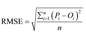

the square root of the mean value of all the squared errors (residuals)

The minimum GCPs that are needed to calculate the RMSE

Minimum of 4

The amount of Residual Error is heavily influenced by this factor.

The quality of GCPs

How does a poorly selected GCP affect RMSE

Causes a higher derived RMSE value

Forward Residual

Shows the error in the same units as the data frame

Inverse Residual

Shows you the error in pixel units

Forward-Inverse Residual

Measure of overall accuracy measured by pixels

Resampling

• During transformation, an empty cell matrix is computed
• Each cell is then given a new value based on its location

Three common methods of Resampling

• Nearest neighbor
• Bilinear interpolation
• Cubic convolution

Nearest Neighbor

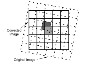• Does not alter original values
• Adopts the value of the nearest pixel
• Best for discrete data (Land use, zoning, roads…)

Two disadvantages of Nearest Neighbor

• Some values may be duplicated or lost
• May result in blocky/disjointed images

Bilinear Interpolation

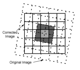• Weighted average of four pixels in the original grid nearest the new pixel
• Creates a new pixel value in the output
• Used for continuous data (Elevation, precipitation…)

Cubic Convolution

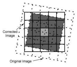• Calculates a distance-weighted average of 16 pixels from the original grid that surrounds the new output pixel.
• Creates a new pixel value in the output
• Used for continuous data
• Elevation, precipitation…

Which Resampling methods are not suited for use with discrete data?

Bilinear Interpolation and Cubic Convolution

What is an advantage of using Bilinear interpolation and Cubic Convolution

They produce sharper image quality and are preferred for remote-sensing data

Spatial analysis

Describes how features are spatially related to one another

Constraints (spatial analysis)

Selections and queries to identify features that meet certain criteria

Proximity (spatial analysis)

How close one feature is to another feature

Networks (spatial analysis)

• What is the shortest route to a location?
• How large of an area can a location serve?

Clustering (spatial analysis)

Are nearby features similar to one another?

Thiessen Polygons

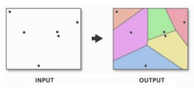a map that shows the area around a point that is closer to that point than any other point

5 step process for making a Thiessen polygon

1. Point data
2. Connect points with thin lines
3. Mark the center point of each line
4. Draw perpendicular lines
5. Erase your thin lines

Buffers

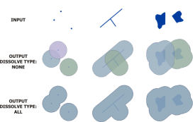• A spatial proximity built around a point, line, or polygon
• Everything that falls within a buffer is within the set distance

• Buffer uses Euclidean distance
• Straight line
• Ignores networks such as roads

Network Analyst

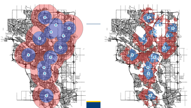• Measured Manhattan Distance
• Analyze routes
• Analyze a service area
• Use distance or time

Manhattan Distance

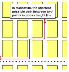• Distance between two points on a grid
• Requires a network (typically, road)

Near

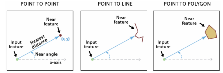• Near features can be points, lines, or polygons
• Measures the distance between input features and near features
• Distance is stored in the input feature

• The Near Tool will add a new attribute field called “near distance”
• Users set a search distance
• No changes in the visual output

Kernel Density (KDE)

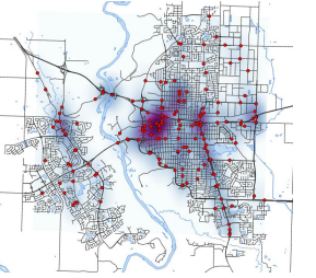•Kernel Density (KDE) calculates the density of point features around each output raster cell
• Creates an output raster and calculates the density of points around each raster cell

Feature types that can be used in KDE

Point and Line Features

Possible uses of KDE

House density, crime reports, roads, wildlife habitat, etc

What does a KDE 'window' do?

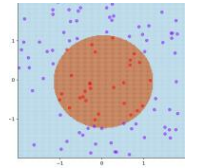Counts the number of points within it to determine the density.

What can fill a Raster Cell

Integers, Real Numbers, or Null (NODATA)

Vertical Datum

baseline used for measuring elevation
• Based on mean sea level determined by the shape of the geoid

Represents elevation on a topographic map

contour lines

For topographic maps to be scanned to create and apply digital elevations, two things are required of the topographic map.

It must be Georeferenced and Digitized

Photogrammetry

Stereo pairs used to calculate elevation manually or digitally

Light Detection and Ranging (LiDAR)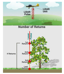

•Emits a laser pulse to the Earth’s surface and measures the return
•Satellite, aircraft, or drone-based
•Accuracy ranges from 3 to 30 cm

Radio Detection and Ranging (Radar)

Emits a radio wave to measure the Earth's surface

Digital Elevation Model (DEM)

Representation of the surface of the Earth

• Bare Earth model
• Does not include features on the surface
• Raster-based approach with one value

Triangulated Irregular Network (TIN)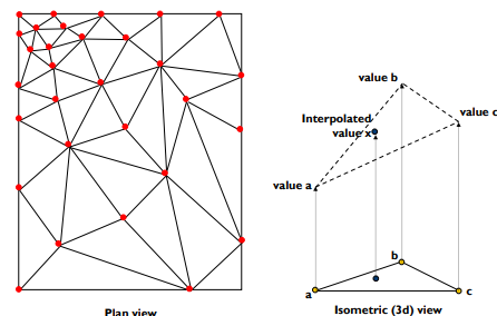

• Vector-based approach to creating Digital Elevation Models
•Allows for non-equally spaced elevation points
•Adjacent points are connected by lines to create a network of nonoverlapping triangles
• Calculate interpolated values between points using trigonometry

Advantages of TIN

• Accepts randomly sampled data
• Displays linear features such as contours and break lines
• Accepts point features (peaks)
• Can vary the density of points according to terrain

Advantages of DEM

• Accepts data directly from a matrix of cells
• Less complex and faster processing

Disadvantages of TIN

• Data intense and longer processing time
• Each vertex stores x, y, z coordinates

Disadvantages of DEM

• Must be resampled if irregular data is used
• May miss complex topography
• May include redundant data in low-relief areas

Digital Surface Model (DSM)

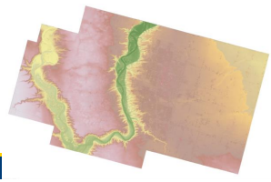• A measurements of ground elevation heights as well as the objects on the ground.
• May be thought of as a full 3-D model of the surface.

Watershed Analysis

• DEMS are used to delineate watersheds, calculate flow accumulation and direction.
•Impacts political agreements, downstream agriculture, and communities.

Predictive Surfaces

Using measurements at a set of locations to predict values in locations that were not measured.

Predictive Surfaces can be used to do two things

Interpolate and/or Extrapolate

Interpolate

is the process of predicting values between known points

Extrapolate

predicts values outside of known sample points

Exact interpolation method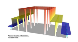

Creates a surface that passes through all known points

Approximate interpolation method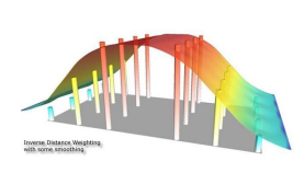

Creates a surface that may vary from known values

Local Interpolation method

Use spatially defined data subsets

Global Interpolation method

Use all data in the study area

4 possible predictive surfaces

• Inverse Distance Weighting (IDW)
• Natural Neighbor
• Spline
• Trend

Inverse Distance Weighting (IDW)

• IDW predicts values using a weighted combination of sample points
• Weight decreases with distance from the grid cell
• Follows an inverse power function
• The Power controls the significance of points based on their distance.
• Increased power puts more emphasis on the nearest points (Default = 2)

Tobler's First law of Geography

“Everything is related to everything else, but near things are more related than
distant things."

Benefits of using IDW

• There is a known influence of proximity
• Uniform distribution of points
• Can control the smoothness

Limitations of IDW

• Doesn’t handle sharp changes in data
• Can create a bullseye pattern around points
• Does not extrapolate

Fixed Search Radius (IDW)

Fixed search radius will remain constant unless a minimum number of points is not met

Variable Search Radius (IDW)

Variable search radius will change to include a minimum number of sample points

Barriers (IDW)

• Breaklines that limit the search for samples
• Cliff or ridge line

Natural Neighbor

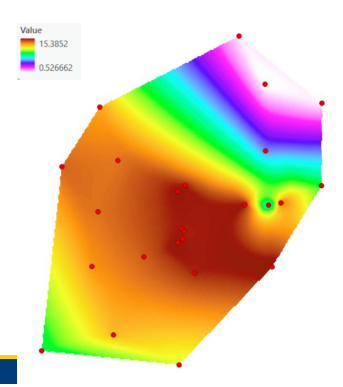• Finds the nearest input samples to a grid cell and weights them based on proportionate areas overlapping the grid cell area.
• Local interpolation
• Exact interpolation

Benefits of Natural Neighbor

• Ideal for irregularly spaced data
• Resistant to cluster bias or overrepresentation

Limitations of Natural Neighbor

• Does not represent peaks, ridges or valleys
• Computationally intensive
• Does not extrapolate

Spline

• Minimizes the curvature to create a smooth surface
• Local interpolation
• Exact interpolation that exceeds the minimum and maximum values

• Users can control the number of points used to calculate each interpolated cell value.
• More points = smoother surface

Benefits of Spline

• Estimates beyond the max & min
• Captures subtle variations
• Best for gently varying surfaces
• Extrapolates based on the last trend

Limitations of Spline

• Can miss sharp changes (cliffs, fault lines…)
• Can create unrealistic values
• Not ideal for dense points with extreme differences

Regularized Spline

allows users to adjust the weight parameter to smooth the surface.
• Higher weight = smoother surface

Tension Spline

allows users to adjust the weight parameter to stiffen the surface.
• Creates a less smooth surface constrained by the sample points.

Overlay

A layer that reveals more information about an underlying map

Trend

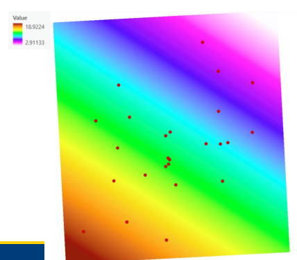• Global polynomial interpolation method used to capture coarse-scale patterns
• Global interpolation
• Approximate interpolation
• Passing a piece of paper through raised points
• Mathematical formulas can increase the “bending” of the s

First order polynomial

linear

Second order polynomial

one bend

Third order polynomial

two bends

Benefits of Trend

• Large-scale pattern recognition
• Extrapolates data

Limitations of Trend

• Oversimplifies data
• Miss local variability
• Inaccurate for small-scale analysis